Stochastic Optimization

Note

If you have not yet set up Python on your computer, you can execute this tutorial in your browser via Google Colab. Click on the rocket in the top right corner and launch “Colab”. If that doesn’t work download the .ipynb file and import it in Google Colab.

Then install the following packages by executing the following command in a Jupyter cell at the top of the notebook.

!pip install pypsa matplotlib highspy

This example demonstrates principles of stochastic optimization for energy system planning under uncertainty and their implementation in PyPSA. See User Guide - Stochastic Optimization. We will consider a stylized capacity expansion model with three scenarios with low, medium, and high gas prices. The network will have a single-bus with a constant load and solar, wind, gas and lignite as extendable generators and the following gas price scenarios:

Scenario	Gas Price	Probability
Low	40 €/MWh	40%
Medium	70 €/MWh	30%
High	100 €/MWh	30%

Import Packages

Let’s first import the necessary packages.

import matplotlib.pyplot as plt
import pandas as pd

import pypsa
from pypsa.common import annuity

Prepare Input Data

Then, we set a few general parameters, load capacity factor time series and techno-economic data such as investment costs and conversion efficiencies.

# Scenario definitions - Gas price uncertainty
SCENARIOS = ["low", "med", "high"]
GAS_PRICES = {"low": 40, "med": 70, "high": 100}  # EUR/MWh_th
PROB = {"low": 0.4, "med": 0.3, "high": 0.3}  # Scenario probabilities
BASE = "low"  # Base scenario for network construction

# System parameters
FREQ = "3h"  # Time resolution
LOAD_MW = 1  # Constant load (MW)
SOLVER = "highs"  # Optimization solver

# Time series data URL
TS_URL = (
    "https://tubcloud.tu-berlin.de/s/pKttFadrbTKSJKF/download/time-series-lecture-2.csv"
)

# Load and process time series data
ts = pd.read_csv(TS_URL, index_col=0, parse_dates=True)
ts = ts.resample(FREQ).asfreq()  # Resample to 3-hour resolution


# Technology data: investment costs, efficiencies, marginal costs
TECH = {
    "solar": {"profile": "solar", "inv": 1e6, "m_cost": 0.01},
    "wind": {"profile": "onwind", "inv": 2e6, "m_cost": 0.02},
    "gas": {"inv": 7e5, "eff": 0.6},
    "lignite": {"inv": 1.3e6, "eff": 0.4, "m_cost": 130},
}

# Financial parameters
FOM, DR, LIFE = 3.0, 0.03, 25  # Fixed O&M (%), discount rate, lifetime (years)

# Calculate annualized capital costs
for cfg in TECH.values():
    cfg["fixed_cost"] = (annuity(DR, LIFE) + FOM / 100) * cfg["inv"]


COLOR_MAP = {
    "solar": "gold",
    "wind": "skyblue",
    "gas": "brown",
    "lignite": "black",
}

Create PyPSA Network

Next, we build the PyPSA network from the provided input data. We wrap it in a function for easy reuse for different scenarios.

def build_network(gas_price: float) -> pypsa.Network:
    n = pypsa.Network()
    n.set_snapshots(ts.index)
    n.snapshot_weightings = pd.Series(int(FREQ[:-1]), index=ts.index)  # 3-hour weights

    # Add bus and load
    n.add("Bus", "DE")
    n.add("Load", "DE_load", bus="DE", p_set=LOAD_MW)

    # Add renewable generators (variable renewable energy)
    for tech in ["solar", "wind"]:
        cfg = TECH[tech]
        n.add(
            "Generator",
            tech,
            bus="DE",
            p_nom_extendable=True,
            p_max_pu=ts[cfg["profile"]],  # Renewable availability profile
            capital_cost=cfg["fixed_cost"],
            marginal_cost=cfg["m_cost"],
        )

    # Add conventional generators (dispatchable)
    for tech in ["gas", "lignite"]:
        cfg = TECH[tech]
        # Gas marginal cost depends on gas price and efficiency
        mc = (gas_price / cfg.get("eff")) if tech == "gas" else cfg["m_cost"]
        n.add(
            "Generator",
            tech,
            bus="DE",
            p_nom_extendable=True,
            efficiency=cfg.get("eff"),
            capital_cost=cfg["fixed_cost"],
            marginal_cost=mc,
        )
    return n

Deterministic Optimization

Initially, let’s solve separate deterministic optimization problems for each gas price scenario. This represents the approach where we assume perfect foresight on the uncertain parameter. That means we solve the problem for each scenario independently.

caps_det = pd.DataFrame(index=SCENARIOS, columns=TECH.keys())
objs_det = pd.Series(index=SCENARIOS)

for sc in SCENARIOS:
    n = build_network(GAS_PRICES[sc])
    n.optimize(solver_name=SOLVER, log_to_console=False)
    caps_det.loc[sc] = n.generators.p_nom_opt
    objs_det.loc[sc] = n.objective

INFO:pypsa.network.index:Applying weightings to all columns of `snapshot_weightings`

WARNING:pypsa.consistency:The following buses have carriers which are not defined:
Index(['DE'], dtype='object', name='name')

INFO:linopy.model: Solve problem using Highs solver

INFO:linopy.model:Solver options:
 - log_to_console: False

INFO:linopy.io:Writing objective.

Writing constraints.:   0%|          | 0/4 [00:00<?, ?it/s]

Writing constraints.: 100%|██████████| 4/4 [00:00<00:00, 42.76it/s]

Writing continuous variables.:   0%|          | 0/2 [00:00<?, ?it/s]

Writing continuous variables.: 100%|██████████| 2/2 [00:00<00:00, 113.35it/s]

INFO:linopy.io: Writing time: 0.13s

INFO:linopy.constants: Optimization successful: 
Status: ok
Termination condition: optimal
Solution: 11684 primals, 26284 duals
Objective: 6.45e+05
Solver model: available
Solver message: Optimal

INFO:pypsa.optimization.optimize:The shadow-prices of the constraints Generator-ext-p-lower, Generator-ext-p-upper were not assigned to the network.

INFO:pypsa.network.index:Applying weightings to all columns of `snapshot_weightings`

WARNING:pypsa.consistency:The following buses have carriers which are not defined:
Index(['DE'], dtype='object', name='name')

INFO:linopy.model: Solve problem using Highs solver

INFO:linopy.model:Solver options:
 - log_to_console: False

INFO:linopy.io:Writing objective.

Writing constraints.:   0%|          | 0/4 [00:00<?, ?it/s]

Writing constraints.: 100%|██████████| 4/4 [00:00<00:00, 43.98it/s]

Writing continuous variables.:   0%|          | 0/2 [00:00<?, ?it/s]

Writing continuous variables.: 100%|██████████| 2/2 [00:00<00:00, 121.17it/s]

INFO:linopy.io: Writing time: 0.13s

INFO:linopy.constants: Optimization successful: 
Status: ok
Termination condition: optimal
Solution: 11684 primals, 26284 duals
Objective: 9.96e+05
Solver model: available
Solver message: Optimal

INFO:pypsa.optimization.optimize:The shadow-prices of the constraints Generator-ext-p-lower, Generator-ext-p-upper were not assigned to the network.

INFO:pypsa.network.index:Applying weightings to all columns of `snapshot_weightings`

WARNING:pypsa.consistency:The following buses have carriers which are not defined:
Index(['DE'], dtype='object', name='name')

INFO:linopy.model: Solve problem using Highs solver

INFO:linopy.model:Solver options:
 - log_to_console: False

INFO:linopy.io:Writing objective.

Writing constraints.:   0%|          | 0/4 [00:00<?, ?it/s]

Writing constraints.: 100%|██████████| 4/4 [00:00<00:00, 47.66it/s]

Writing continuous variables.:   0%|          | 0/2 [00:00<?, ?it/s]

Writing continuous variables.: 100%|██████████| 2/2 [00:00<00:00, 124.48it/s]

INFO:linopy.io: Writing time: 0.12s

INFO:linopy.constants: Optimization successful: 
Status: ok
Termination condition: optimal
Solution: 11684 primals, 26284 duals
Objective: 1.11e+06
Solver model: available
Solver message: Optimal

INFO:pypsa.optimization.optimize:The shadow-prices of the constraints Generator-ext-p-lower, Generator-ext-p-upper were not assigned to the network.

# Visualize deterministic results
fig, (ax1, ax2) = plt.subplots(1, 2, figsize=(14, 5))

colors = [COLOR_MAP.get(c, "gray") for c in caps_det.columns]
caps_det.plot(kind="bar", stacked=True, ax=ax1, color=colors)
ax1.set_title("Deterministic Capacity Mix by Scenario")
ax1.set_ylabel("Capacity (MW)")
ax1.legend(loc="upper left")

(objs_det / 1e6).plot(kind="bar", ax=ax2, color="steelblue")
ax2.set_title("Deterministic Total Costs by Scenario")
ax2.set_ylabel("Total Cost (M€/year)")

Text(0, 0.5, 'Total Cost (M€/year)')

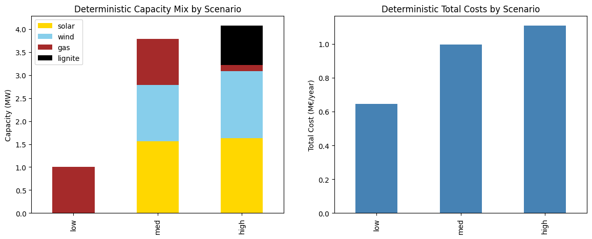
We observe that higher gas prices lead to more renewable capacity expansion and less gas capacity. As gas prices increase, total system costs rise.

n.model

Linopy LP model
===============

Variables:
----------
 * Generator-p_nom (name)
 * Generator-p (snapshot, name)

Constraints:
------------
 * Generator-ext-p_nom-lower (name)
 * Generator-ext-p-lower (snapshot, name)
 * Generator-ext-p-upper (snapshot, name)
 * Bus-nodal_balance (name, snapshot)

Status:
-------
ok

Stochastic Optimization

The key to stochastic optimization in PyPSA is the n.set_scenarios() method. This method transforms a regular PyPSA network into a stochastic network by adding scenario dimensions to all component data which allows specifying scenario-specific parameters. Once scenarios are set, PyPSA treats investment decisions as first-stage variables that must be the same across all scenarios, while dispatch decisions become second-stage variables that can differ by scenario.

We start by building a deterministic network for our (arbitrarily selected) base scenario. Subsequently, we add our scenarios to the network.

n_stoch = build_network(GAS_PRICES[BASE])
n_stoch.set_scenarios(PROB)

INFO:pypsa.network.index:Applying weightings to all columns of `snapshot_weightings`

After that, we can set the scenario-specific parameters, i.e. the varying gas prices by scenario.

for sc in SCENARIOS:
    n_stoch.generators.loc[(sc, "gas"), "marginal_cost"] = (
        GAS_PRICES[sc] / n_stoch.generators.loc[(sc, "gas"), "efficiency"]
    )

n_stoch.generators.xs("gas", level="name").marginal_cost

scenario
low      66.666667
med     116.666667
high    166.666667
Name: marginal_cost, dtype: float64

Now, we can solve the stochastic optimisation model:

n_stoch.optimize(solver_name=SOLVER, log_to_console=False)

print(f"Total expected cost: {n_stoch.objective / 1e6:.3f} M€/year")

caps_api = n_stoch.generators.p_nom_opt.xs(BASE, level="scenario")
obj_api = n_stoch.objective

WARNING:pypsa.consistency:The following buses have carriers which are not defined:
MultiIndex([( 'low', 'DE'),
            ( 'med', 'DE'),
            ('high', 'DE')],
           names=['scenario', 'name'])

INFO:linopy.model: Solve problem using Highs solver

INFO:linopy.model:Solver options:
 - log_to_console: False

INFO:linopy.io:Writing objective.

Writing constraints.:   0%|          | 0/4 [00:00<?, ?it/s]

Writing constraints.:  75%|███████▌  | 3/4 [00:00<00:00, 15.57it/s]

Writing constraints.: 100%|██████████| 4/4 [00:00<00:00, 16.19it/s]

Writing continuous variables.:   0%|          | 0/2 [00:00<?, ?it/s]

Writing continuous variables.: 100%|██████████| 2/2 [00:00<00:00, 41.67it/s]

INFO:linopy.io: Writing time: 0.34s

INFO:linopy.constants: Optimization successful: 
Status: ok
Termination condition: optimal
Solution: 35044 primals, 78852 duals
Objective: 9.69e+05
Solver model: available
Solver message: Optimal

INFO:pypsa.optimization.optimize:The shadow-prices of the constraints Generator-ext-p-lower, Generator-ext-p-upper were not assigned to the network.

Total expected cost: 0.969 M€/year

n_stoch.model

Linopy LP model
===============

Variables:
----------
 * Generator-p_nom (name)
 * Generator-p (scenario, name, snapshot)

Constraints:
------------
 * Generator-ext-p_nom-lower (name, scenario)
 * Generator-ext-p-lower (scenario, name, snapshot)
 * Generator-ext-p-upper (scenario, name, snapshot)
 * Bus-nodal_balance (name, scenario, snapshot)

Status:
-------
ok

caps_comparison = caps_det.copy()
caps_comparison.loc["Stochastic"] = caps_api

objs_comparison = objs_det.copy()
objs_comparison.loc["Stochastic"] = obj_api

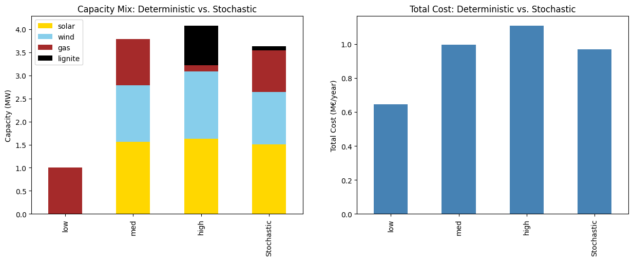
fig, (ax1, ax2) = plt.subplots(1, 2, figsize=(15, 5))

colors = [COLOR_MAP.get(c, "gray") for c in caps_comparison.columns]
caps_comparison.plot(kind="bar", stacked=True, ax=ax1, color=colors)
ax1.set_title("Capacity Mix: Deterministic vs. Stochastic")
ax1.set_ylabel("Capacity (MW)")
ax1.legend(loc="upper left")

(objs_comparison / 1e6).plot(kind="bar", ax=ax2, color="steelblue")
ax2.set_title("Total Cost: Deterministic vs. Stochastic")
ax2.set_ylabel("Total Cost (M€/year)")

Text(0, 0.5, 'Total Cost (M€/year)')

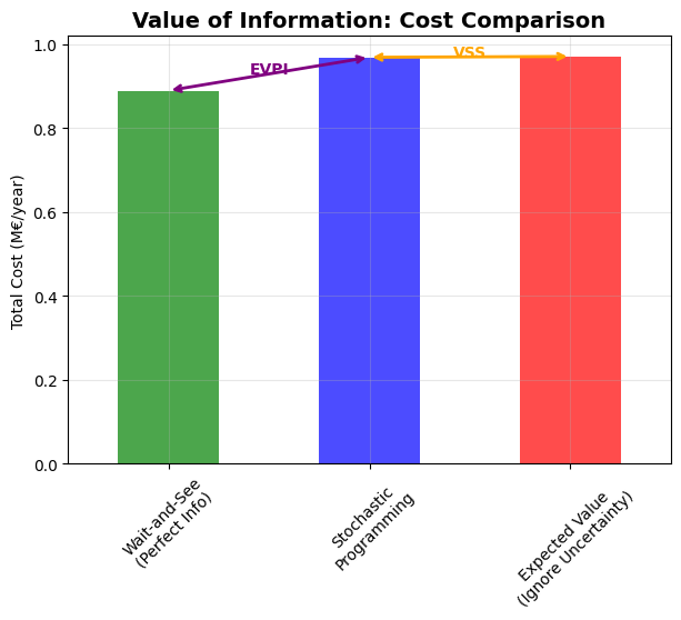
Value of Information Metrics

We can also now calculate the Value of Information (VoI) metrics, which include the Expected Value of Perfect Information (EVPI) and the Value of Stochastic Solution (VSS). These metrics help us understand the benefits of incorporating uncertainty into our optimization model.

# Wait-and-See (perfect information) expected cost
ws_cost = sum(objs_det[sc] * PROB[sc] for sc in SCENARIOS)
print(f"Wait-and-See (WS) cost: {ws_cost / 1e6:.3f} M€/year")

Wait-and-See (WS) cost: 0.890 M€/year

# Expected Value of Perfect Information
evpi = obj_api - ws_cost
print(f"EVPI (SP - WS): {evpi / 1e6:.3f} M€/year")

EVPI (SP - WS): 0.079 M€/year

# Expected gas price
expected_gas_price = sum(GAS_PRICES[sc] * PROB[sc] for sc in SCENARIOS)
print(f"Expected gas price: {expected_gas_price:.1f} EUR/MWh_th")

Expected gas price: 67.0 EUR/MWh_th

# Report stochastic programming (SP) cost
print(f"Stochastic Prog (SP) cost: {obj_api / 1e6:.3f} M€/year")

Stochastic Prog (SP) cost: 0.969 M€/year

# Solve deterministic problem with expected gas price (EEV solution)
n_eev = build_network(expected_gas_price)
n_eev.optimize(solver_name=SOLVER, log_to_console=False)
eev_capacities = n_eev.generators.p_nom_opt

# Evaluate EEV capacities under each scenario
eev_costs = []
for sc in SCENARIOS:
    n_eval = build_network(GAS_PRICES[sc])
    for tech in TECH.keys():
        n_eval.generators.loc[tech, "p_nom_max"] = eev_capacities[tech]
        n_eval.generators.loc[tech, "p_nom_min"] = eev_capacities[tech]
    n_eval.optimize(solver_name=SOLVER, log_to_console=False)
    eev_costs.append(n_eval.objective)

eev_expected_cost = sum(eev_costs[i] * PROB[sc] for i, sc in enumerate(SCENARIOS))
print(f"Expected Value (EEV) cost: {eev_expected_cost / 1e6:.3f} M€/year")

INFO:pypsa.network.index:Applying weightings to all columns of `snapshot_weightings`

WARNING:pypsa.consistency:The following buses have carriers which are not defined:
Index(['DE'], dtype='object', name='name')

INFO:linopy.model: Solve problem using Highs solver

INFO:linopy.model:Solver options:
 - log_to_console: False

INFO:linopy.io:Writing objective.

Writing constraints.:   0%|          | 0/4 [00:00<?, ?it/s]

Writing constraints.: 100%|██████████| 4/4 [00:00<00:00, 45.45it/s]

Writing continuous variables.:   0%|          | 0/2 [00:00<?, ?it/s]

Writing continuous variables.: 100%|██████████| 2/2 [00:00<00:00, 116.40it/s]

INFO:linopy.io: Writing time: 0.12s

INFO:linopy.constants: Optimization successful: 
Status: ok
Termination condition: optimal
Solution: 11684 primals, 26284 duals
Objective: 9.71e+05
Solver model: available
Solver message: Optimal

INFO:pypsa.optimization.optimize:The shadow-prices of the constraints Generator-ext-p-lower, Generator-ext-p-upper were not assigned to the network.

INFO:pypsa.network.index:Applying weightings to all columns of `snapshot_weightings`

WARNING:pypsa.consistency:The following buses have carriers which are not defined:
Index(['DE'], dtype='object', name='name')

INFO:linopy.model: Solve problem using Highs solver

INFO:linopy.model:Solver options:
 - log_to_console: False

INFO:linopy.io:Writing objective.

Writing constraints.:   0%|          | 0/5 [00:00<?, ?it/s]

Writing constraints.: 100%|██████████| 5/5 [00:00<00:00, 55.47it/s]

Writing continuous variables.:   0%|          | 0/2 [00:00<?, ?it/s]

Writing continuous variables.: 100%|██████████| 2/2 [00:00<00:00, 123.01it/s]

INFO:linopy.io: Writing time: 0.12s

INFO:linopy.constants: Optimization successful: 
Status: ok
Termination condition: optimal
Solution: 11684 primals, 26288 duals
Objective: 7.37e+05
Solver model: available
Solver message: Optimal

INFO:pypsa.optimization.optimize:The shadow-prices of the constraints Generator-ext-p-lower, Generator-ext-p-upper were not assigned to the network.

INFO:pypsa.network.index:Applying weightings to all columns of `snapshot_weightings`

WARNING:pypsa.consistency:The following buses have carriers which are not defined:
Index(['DE'], dtype='object', name='name')

INFO:linopy.model: Solve problem using Highs solver

INFO:linopy.model:Solver options:
 - log_to_console: False

INFO:linopy.io:Writing objective.

Writing constraints.:   0%|          | 0/5 [00:00<?, ?it/s]

Writing constraints.: 100%|██████████| 5/5 [00:00<00:00, 56.03it/s]

Writing continuous variables.:   0%|          | 0/2 [00:00<?, ?it/s]

Writing continuous variables.: 100%|██████████| 2/2 [00:00<00:00, 116.03it/s]

INFO:linopy.io: Writing time: 0.12s

INFO:linopy.constants: Optimization successful: 
Status: ok
Termination condition: optimal
Solution: 11684 primals, 26288 duals
Objective: 9.97e+05
Solver model: available
Solver message: Optimal

INFO:pypsa.optimization.optimize:The shadow-prices of the constraints Generator-ext-p-lower, Generator-ext-p-upper were not assigned to the network.

INFO:pypsa.network.index:Applying weightings to all columns of `snapshot_weightings`

WARNING:pypsa.consistency:The following buses have carriers which are not defined:
Index(['DE'], dtype='object', name='name')

INFO:linopy.model: Solve problem using Highs solver

INFO:linopy.model:Solver options:
 - log_to_console: False

INFO:linopy.io:Writing objective.

Writing constraints.:   0%|          | 0/5 [00:00<?, ?it/s]

Writing constraints.: 100%|██████████| 5/5 [00:00<00:00, 53.64it/s]

Writing continuous variables.:   0%|          | 0/2 [00:00<?, ?it/s]

Writing continuous variables.: 100%|██████████| 2/2 [00:00<00:00, 116.85it/s]

INFO:linopy.io: Writing time: 0.13s

INFO:linopy.constants: Optimization successful: 
Status: ok
Termination condition: optimal
Solution: 11684 primals, 26288 duals
Objective: 1.26e+06
Solver model: available
Solver message: Optimal

INFO:pypsa.optimization.optimize:The shadow-prices of the constraints Generator-ext-p-lower, Generator-ext-p-upper were not assigned to the network.

Expected Value (EEV) cost: 0.971 M€/year

# Value of Stochastic Solution
vss = eev_expected_cost - obj_api
print(f"VSS (EEV - SP): {vss / 1e6:.3f} M€/year")

VSS (EEV - SP): 0.002 M€/year

print("\nTheoretical Ordering Check:")
print(f"  WS ≤ SP: {ws_cost <= obj_api} ({ws_cost:.0f} ≤ {obj_api:.0f})")
print(
    f"  SP ≤ EEV: {obj_api <= eev_expected_cost} ({obj_api:.0f} ≤ {eev_expected_cost:.0f})"
)
print(f"  EVPI ≥ 0: {evpi >= 0} ({evpi:.0f} ≥ 0)")
print(f"  VSS ≥ 0: {vss >= 0} ({vss:.0f} ≥ 0)")

Theoretical Ordering Check:
  WS ≤ SP: True (889596 ≤ 968918)
  SP ≤ EEV: True (968918 ≤ 970853)
  EVPI ≥ 0: True (79322 ≥ 0)
  VSS ≥ 0: True (1935 ≥ 0)

costs_voi = pd.Series(
    {
        "Wait-and-See\n(Perfect Info)": ws_cost,
        "Stochastic\nProgramming": obj_api,
        "Expected Value\n(Ignore Uncertainty)": eev_expected_cost,
    }
)


fig, ax1 = plt.subplots(figsize=(7, 5))

# Cost comparison
(costs_voi / 1e6).plot(kind="bar", ax=ax1, color=["green", "blue", "red"], alpha=0.7)
ax1.set_title("Value of Information: Cost Comparison", fontsize=14, fontweight="bold")
ax1.set_ylabel("Total Cost (M€/year)")
ax1.tick_params(axis="x", rotation=45)
ax1.grid(True, alpha=0.3)

# Add EVPI and VSS arrows
ax1.annotate(
    "",
    xy=(0, ws_cost / 1e6),
    xytext=(1, obj_api / 1e6),
    arrowprops={"arrowstyle": "<->", "color": "purple", "lw": 2},
)
ax1.text(
    0.5,
    (ws_cost + obj_api) / (2 * 1e6),
    "EVPI",
    color="purple",
    fontweight="bold",
    fontsize=10,
    ha="center",
)

ax1.annotate(
    "",
    xy=(1, obj_api / 1e6),
    xytext=(2, eev_expected_cost / 1e6),
    arrowprops={"arrowstyle": "<->", "color": "orange", "lw": 2},
)
ax1.text(
    1.5,
    (eev_expected_cost + obj_api) / (2 * 1e6),
    "VSS",
    color="orange",
    fontweight="bold",
    fontsize=10,
    ha="center",
)

Text(1.5, 0.9698854088263178, 'VSS')

References

[1] Birge, J. R., & Louveaux, F. (2011). Introduction to Stochastic Programming.

[2] Birge, J. R. (1982). The value of the stochastic solution in stochastic linear programs with fixed recourse. Mathematical Programming, 24(1), 314-325.