Clustering the network#
Note
If you have not yet set up Python on your computer, you can execute this tutorial in your browser via Google Colab. Click on the rocket in the top right corner and launch “Colab”. If that doesn’t work download the .ipynb file and import it in Google Colab.
Then install the following packages by executing the following command in a Jupyter cell at the top of the notebook.
!pip install cartopy folium geopandas pandas pypsa mapclassify matplotlib numpy shapely
In this notebook, we show how both PyPSA and PyPSA-Eur handle spatial clustering of networks.
Background#
Motivation#
Base network contains more than 6700 buses, of which around 4900 are based on real OSM substation polygons, 1800 are “virtual” buses (the latter needed to model lines that are directly connected to other lines without substations)
Solving an investment and operation model at this regional scale, up to hourly resolution and including sectors beyond electricity is computationally not feasible
Depending on the focus region of interest, both the PyPSA framework and PyPSA-Eur model enable a variety of established clustering algorithms
All components within a bus region will be aggregated and mapped, accordingly
Clustering options#
PyPSA & PyPSA-Eur
By total number of regions, i.e.:
Hierarchical Agglomerative Clustering (HAC)
K-Means
Greedy Modularity, see Frysztacki et al. (2022)
By custom busmap, i.e., providing a dictionary that maps each individual bus to a bus region/group
PyPSA-Eur
By administrative regions, i.e. NUTS0-NUTS3 for EU member status and ADM0-ADM1 for non-EU member states.
Underneath, all clustering methods harness the built-in clustering by busmap. Any clustering method, including HAC, k-means, or by administrative regions, calculates individual busmaps
Exploring the clustering methods#
For execution of the notebook in Google Colab, comment out and run:
# !pip install cartopy folium geopandas pandas pypsa mapclassify matplotlib numpy shapely
Note that in PyPSA-Eur, all of these steps are built into the cluster_network Snakemake rule. For illustrative purposes, we go through the underlying functions, step by step in this notebook. First, we import the example PyPSA network file and built-in functions from the PyPSA package.
import pandas as pd
import pypsa
resources = "https://raw.githubusercontent.com/resilient-project/pypsa-workshop/main/pypsa-workshop/resources/"
n = pypsa.Network(resources + "base.nc")
INFO:pypsa.io:Retrieving network data from https://raw.githubusercontent.com/resilient-project/pypsa-workshop/main/pypsa-workshop/resources/base.nc
WARNING:pypsa.io:Importing network from PyPSA version v0.33.2 while current version is v0.34.1. Read the release notes at https://pypsa.readthedocs.io/en/latest/release_notes.html to prepare your network for import.
INFO:pypsa.io:Imported network base.nc has buses, carriers, lines, links, shapes, transformers
Clustering by K-Means#
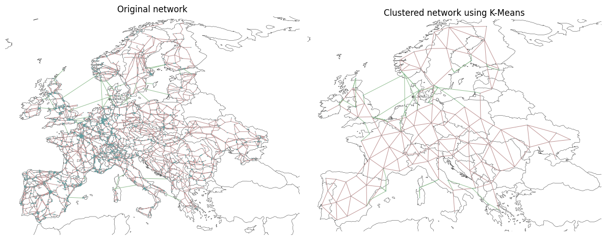
In this first example, we make a clustering based on the K-Means algorithm. We prepare a busmap weighting all original buses, equally. We want to cluster Europe to a 150 nodes.
weighting = pd.Series(1, n.buses.index)
print(weighting.head())
Bus
way/150003587-400     1
way/150003587-220     1
way/174609198-220     1
way/249066440-400     1
way/1302364573-220    1
dtype: int64
We use the imported spatial clustering functions to build the K-Means-based busmap.
busmap_kmeans = n.cluster.busmap_by_kmeans(bus_weightings=weighting, n_clusters=90)
Let’s double-check if all buses have been mapped correctly in the busmap
print(busmap_kmeans.head())
# Unique reqions
print(f"\nUnique values/regions: {len(busmap_kmeans.unique())}")
Bus
way/150003587-400     71
way/150003587-220     71
way/174609198-220     71
way/249066440-400     42
way/1302364573-220    71
dtype: object

Unique values/regions: 90
Now, use built-in PyPSA functions to cluster the network using the calculated busmap
# nc_kmeans = n.cluster.cluster_by_busmap(busmap_kmeans)
What happened? Note that PyPSA by default will throw an error when trying to cluster buses where the carrier attribute does not agree. Specifically, AC and DC buses cannot be clustered by default. So let’s correct our busmap to keep DC buses separate. Note that PyPSA-Eur has built-in steps to mitigate this.
b_dc = n.buses.loc[n.buses.carrier == "DC"].index
Then we make them unique by giving them an individual suffix.
busmap_kmeans.loc[b_dc] = busmap_kmeans.loc[b_dc].astype(str) + "_DC"
Now let’s try clustering again. Note that our number of unique bus regions has increased from the above operation.
print(f"Number of bus regions: {len(busmap_kmeans.unique())}")
Number of bus regions: 119
PyPSA will go through all attributes of the modelled components and throw an error similar to the above, if the attributes do not agree. For illustrative purposes, we ignore the remaining attributes in this notebook.
n.buses = n.buses.reindex(columns=n.components["Bus"]["attrs"].index[1:])
n.lines = n.lines.reindex(columns=n.components["Line"]["attrs"].index[1:])
n.lines["type"] = "Example"
nc_kmeans = n.cluster.cluster_by_busmap(busmap_kmeans)
Let’s explore the clustered network.
nc_kmeans.plot.explore()
INFO:pypsa.plot.maps.interactive:Components rendered on the map: Bus, Line, Link.
INFO:pypsa.plot.maps.interactive:Components omitted as they are missing or not selected: Generator, Load, StorageUnit, Transformer.
… and visualise them side-by-side
import cartopy.crs as ccrs
import matplotlib.pyplot as plt

fig, (ax, ax1) = plt.subplots(
    1, 2, subplot_kw={"projection": ccrs.EqualEarth()}, figsize=(12, 12)
)
plot_kwrgs = dict(bus_sizes=5e-3, line_widths=0.7, link_widths=0.7)
n.plot.map(ax=ax, title="Original network", **plot_kwrgs)
nc_kmeans.plot.map(ax=ax1, title="Clustered network using K-Means", **plot_kwrgs)
fig.tight_layout()
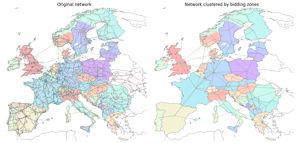
Clustering by bidding zones#
First, we import world bidding zones from a public github repository and import it as GeoDataFrame.
import geopandas as gpd
import numpy as np

world_bz = gpd.read_file(
    "https://raw.githubusercontent.com/electricitymaps/electricitymaps-contrib/v1.238.0/web/geo/world.geojson"
)
We only need Europe in this example.
countries = [
    "AL",
    "AT",
    "BA",
    "BE",
    "BG",
    "CH",
    "CZ",
    "DE",
    "DK",
    "EE",
    "ES",
    "FI",
    "FR",
    "GB",
    "GR",
    "HR",
    "HU",
    "IE",
    "IT",
    "LT",
    "LU",
    "LV",
    "ME",
    "MK",
    "NL",
    "NO",
    "PL",
    "PT",
    "RO",
    "RS",
    "SE",
    "SI",
    "SK",
    "XK",
]
europe_bz = world_bz[world_bz["countryKey"].isin(countries)]

# Remove geometries that are south and east of Portugal
europe_bz = europe_bz[
    (europe_bz.geometry.bounds["minx"] > -12) & (europe_bz.geometry.bounds["maxy"] > 33)
]

europe_bz.head()
| zoneName | countryKey | countryName | geometry | |
|---|---|---|---|---|
| 0 | SE-SE4 | SE | Sweden | MULTIPOLYGON (((12.37512 56.91149, 12.35227 56... |
| 1 | SE-SE3 | SE | Sweden | MULTIPOLYGON (((18.56359 60.22731, 18.32958 60... |
| 2 | SE-SE2 | SE | Sweden | MULTIPOLYGON (((20.3096 63.65475, 20.072 63.66... |
| 3 | SE-SE1 | SE | Sweden | MULTIPOLYGON (((16.38861 67.04356, 16.40663 67... |
| 7 | AL | AL | Albania | MULTIPOLYGON (((20.56881 41.87367, 20.50041 42... |
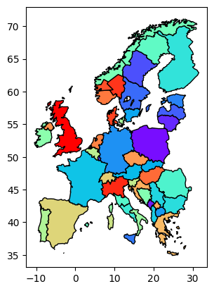
Let’s store all bidding zones in a variable and give them a random order to prepare for plotting.
bidding_zones = europe_bz["zoneName"].unique()
np.random.shuffle(bidding_zones)
import matplotlib.pyplot as plt
import matplotlib.colors as mcolors

# Map each countrykey to a distinct color from the colormap
cmap = plt.colormaps["rainbow"]
norm = mcolors.Normalize(vmin=0, vmax=len(bidding_zones) - 1)

color_dict = {key: cmap(norm(i)) for i, key in enumerate(bidding_zones)}
europe_bz.loc[:, "color"] = europe_bz["zoneName"].map(color_dict)
europe_bz["color"] = europe_bz["color"].apply(
    lambda x: mcolors.to_hex(x)
)  # Hex conversion optional

europe_bz.plot(color=europe_bz["color"], edgecolor="black")
plt.show()
Next, we want to create a custom busmap based on the Polygons contained in the europe_bz GeoDataFrame. For this purpose, we create a GDF from n.buses first.
# Using sjoin_nearest
buses = gpd.GeoDataFrame(
    n.buses,
    geometry=gpd.points_from_xy(n.buses.x, n.buses.y),
    crs="EPSG:4326",
)
We convert both GDFs to a distance-based projection.
distance_crs = "EPSG:3857"
buses = buses.to_crs(distance_crs)
europe_bz = europe_bz.to_crs(distance_crs)
Now we can use GeoPandas sjoin_nearest() function to map each network bus to a corresponding bidding zone.
# Using sjoin_nearest map to europe_bz
buses_mapped = gpd.sjoin_nearest(
    buses[["geometry"]],
    europe_bz[["zoneName", "geometry"]],
    how="left",
    lsuffix="bus",
    rsuffix="bz",
)

busmap_bz = buses_mapped["zoneName"]
We use PyPSA’s clustering by busmap functionalities again to cluster by our custom busmap. This time, we want all buses to be clustered together, independent of their carrier attribute. AC and DC buses should be mapped to the same geographic regions.
n.buses["carrier"] = "AC"  # We turn all DC buses into AC

nc_bz = n.cluster.cluster_by_busmap(busmap_bz)
Again, we compare them side-by-side:
# set bounds
europe_bz_latlon = europe_bz.to_crs(epsg=4326)
bounds = europe_bz_latlon.total_bounds  # returns [minx, miny, maxx, maxy]

fig, (ax, ax1) = plt.subplots(
    1, 2, subplot_kw={"projection": ccrs.EqualEarth()}, figsize=(12, 12)
)

plot_kwrgs = dict(bus_sizes=5e-3, line_widths=0.7, link_widths=0.7)
n.plot(ax=ax, title="Original network", **plot_kwrgs)

# Adding the bidding zones
europe_bz.to_crs(epsg=8857).plot(ax=ax, color=europe_bz["color"], alpha=0.3)
europe_bz.to_crs(epsg=8857).plot(ax=ax1, color=europe_bz["color"], alpha=0.3)
nc_bz.plot(ax=ax1, title="Network clustered by bidding zones", **plot_kwrgs)

ax.set_extent([bounds[0], bounds[2], bounds[1], bounds[3]], crs=ccrs.PlateCarree())
ax1.set_extent([bounds[0], bounds[2], bounds[1], bounds[3]], crs=ccrs.PlateCarree())

fig.tight_layout()
/tmp/ipykernel_2162/1969779938.py:10: DeprecatedWarning:

plot is deprecated. Use `n.plot.map()` as a drop-in replacement instead.
/tmp/ipykernel_2162/1969779938.py:15: DeprecatedWarning:

plot is deprecated. Use `n.plot.map()` as a drop-in replacement instead.
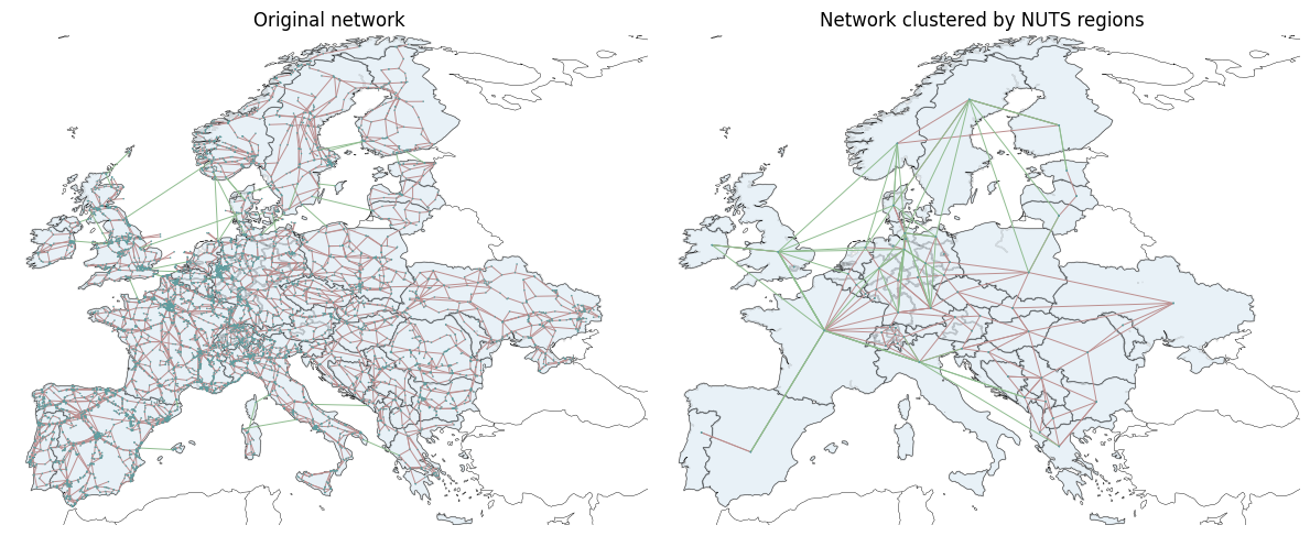
Clustering by administrative regions#
PyPSA-Eur has a built-in function to set administrative clustering level for each country, individually. To get the clustered network below, set:
config.yaml
scenario:
  clusters:
  - adm

clustering:
  mode: administrative
  administrative:
    level: 0
    DE: 1
    BE: 1
    AT: 1
    CH: 2
We import the network and administrative shape file for illustrative purposes
nc_adm = pypsa.Network(resources + "base_s_adm_elec_.nc")
admin_shapes = gpd.read_file(resources + "admin_shapes.geojson")
INFO:pypsa.io:Retrieving network data from https://raw.githubusercontent.com/resilient-project/pypsa-workshop/main/pypsa-workshop/resources/base_s_adm_elec_.nc
WARNING:pypsa.io:Importing network from PyPSA version v0.33.2 while current version is v0.34.1. Read the release notes at https://pypsa.readthedocs.io/en/latest/release_notes.html to prepare your network for import.
INFO:pypsa.io:Imported network base_s_adm_elec_.nc has buses, carriers, generators, lines, links, loads, storage_units, stores
# set bounds
bounds = admin_shapes.total_bounds  # returns [minx, miny, maxx, maxy]

fig, (ax, ax1) = plt.subplots(
    1, 2, subplot_kw={"projection": ccrs.EqualEarth()}, figsize=(12, 12)
)

plot_kwrgs = dict(bus_sizes=5e-3, line_widths=0.7, link_widths=0.7)
n.plot.map(ax=ax, title="Original network", **plot_kwrgs)

# Adding the bidding zones
admin_shapes.to_crs(epsg=8857).plot(ax=ax, alpha=0.1, edgecolor="black")
admin_shapes.to_crs(epsg=8857).plot(ax=ax1, alpha=0.1, edgecolor="black")
nc_adm.plot.map(ax=ax1, title="Network clustered by NUTS regions", **plot_kwrgs)

ax.set_extent([bounds[0], bounds[2], bounds[1], bounds[3]], crs=ccrs.PlateCarree())
ax1.set_extent([bounds[0], bounds[2], bounds[1], bounds[3]], crs=ccrs.PlateCarree())

fig.tight_layout()
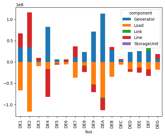
As this is a solved network, we can also inspect solutions for each individual NUTS region by their unique identifier, e.g.
nc_adm.statistics.energy_balance(
    groupby="bus", comps=["Generator", "Load", "Link", "Line", "Store", "StorageUnit"]
).filter(like="DE").unstack().T.plot(kind="bar", stacked=True)
<Axes: xlabel='bus'>
References#
Frysztacki, M.M., Recht, G. & Brown, T. A comparison of clustering methods for the spatial reduction of renewable electricity optimisation models of Europe. Energy Inform 5, 4. https://doi.org/10.1186/s42162-022-00187-7 (2022).
Hörsch, J., Hofmann, F., Schlachtberger, D. & Brown, T. PyPSA-Eur: An open optimisation model of the European transmission system. Energy Strategy Reviews 22, 207–215, https://doi.org/10.1016/j.esr.2018.08.012 (2018).